Overview

I’ve recently been working on improving the lighting for my renderer, and a part of that improvement has been updating my image based lighting implementation. In this article, I’ll give you an overview of the lighting model I’m using and how I compute irradiance maps and pre-filtered environment maps in real time.

PBR Rendering

My renderer, like most modern renderers, is physically based. In non-technical terms that means that the techniques I’m using to compute lighting are attempting to look as physically plausable as possible. In more technical terms that means:

1. It’s based on micro-facets/micro-geometry.
2. It’s using a physically based BRDF.
3. It’s energy conserving.

The Micro-facet model is a way of describing surfaces. We assume that no surface is perfectly smooth, and are instead made of many tiny perfect mirrors. When light rays bounce off of these mirrors they scatter, producing the visual effect of a surface. The more aligned these mirrors are, the smoother the surface appears. The more chaotic the mirrors, the more the rays bounce randomly, giving the appearance of a rough surface. We approximate these surfaces using a statistical model, since it’s not feasible to actually model surfaces using the billions of mirrors required in real time.

A Figure from Real-Time Rendering (4th Edition) showing micro-facets.

“Energy conserving” in the context of the micro-facet model simply means that the outgoing light energy bounced off a surface should never exceed the incoming light energy.

The “BRDF” is a component of the rendering equation.

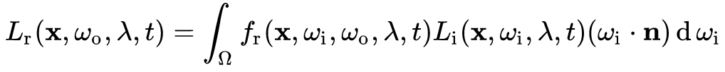The rendering equation from Wikipedia.

The integral looks pretty scary at first, but really all it’s saying is that the light we observe at a location x when looking from a direction ω0 is equal to all the incoming light to that point over a hemisphere centered around the surface normal n weighted by the BRDF fr.

The two resources I used to learn about this were the Learn OpenGL articles on PBR rendering and Real-Time Rendering (4th Edition). The Learn OpenGL articles are much more practical if all you care about are implementation details, but Real-Time Rendering goes into much more detail about the mathematics and covers many more topics that Learn OpenGL doesn’t (subsurface scattering and cloth rendering, for example).

The Cook-Torrance BRDF

It’s common to split up the lighting contributions into different parts. Specifically, using the Cook-Torrance BRDF, we split up the equation into a diffuse portion and a specular portion. The equation looks like this:

The Cook-Torrance BRDF from Learn OpenGL.

The specular portion (weighted by ks) is the light that is reflected off the surface. The diffuse portion (weighted by kd) is the light that gets refracted into the surface, bounces around, and then exits the surface in random directions. The specular portion is what gives you pretty reflections and the diffuse portion is what gives you rough surfaces. Note that kd + ks = 1 if we want to conserve energy. The f components are themselves functions, but the specifics aren’t entirely relevant here, so I will skip over them. If you’re curious, the article I linked earlier by Learn OpenGL provides a good explanation.

Global Illumination

So, physically based rendering is sick. You can plug in your lights, materials, and models and everything will look nice. However, there is a particular portion of lighting that is very difficult to compute accurately in real time: ambient lighting. Or, if you’d like to be more fancy about it, global illumination. This is all the lighting that doesn’t come from light rays going directly from the light source to the surface. Or, in other words, it’s the light that bounces around. Global illumination (GI for short) is very important for making the lighting of a scene look realistic, and a lot of research is currently being done to get it computed in real time. If you’re curious here are some talks by Epic Games and Electronic Arts on their techniques for realtime GI. Here is a comparison image of a scene with and without GI.

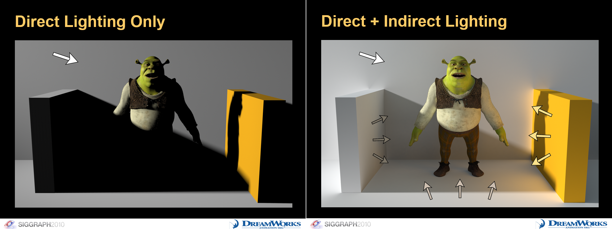A figure from this article which, itself, is from Tabellion, E. “Ray Tracing vs. Point-Based GI for Animated Films”. SIGGRAPH 2010 Course: “Global Illumination Across Industries”. Available Online.

So, why is GI so hard to compute in real time? It has to do with a combination of two things.

First, for real time rendering, we typically only care about the color of things that are on screen. We don’t want to waste time doing lighting calculations for pixels that are never going to be seen. However, GI breaks this, because suddenly we need to know about the lighting on nearby surfaces that might be off screen because they might bounce light onto surfaces that are on screen.

Computing this bounce lighting accurately requires ray tracing which brings us to the second reason why GI is hard to do in real time: ray tracing is SOOOO SLOOOW! Why? Consider a typical scene. The Amazon Lumberyard Bistro scene that I like to use for testing has about 2.8 million triangles on the exterior. In order to see if a ray hits a surface you have to check it against each individual triangle. According to the Epic Games presentation I linked earlier, they found that 100 rays per pixel are needed for good results in exterior scenes. If you’re rendering at 1080p, that ends up being about 580.6 trillion operations for a single bounce. That’s insane. You can reduce the number of triangles you have to check by organizing your objects into an acceleration structure (typically a BVH), but this still isn’t enough to give you the speed for 100 rays per pixel.

Image Based Lighting

This brings us to image based lighting. This is an approximation (and I’m using approximation in the loosest of terms here) for GI where we treat the surrounding environment as a light. In my case, by “the surrounding environment”, I mean the sky box. This technique is nowhere near the quality of realtime GI, but it’s fast and looks way better than having a flat color for ambient lighting (which was common practice for a long while).

In image based lighting, we store environmental lighting in two cube maps. The first is called an irradiance map. This captures the diffuse reflections from our environment. The second is called a pre-filtered environment map, and this is used for specular reflections. I’ll go over each and describe how I generate these every frame.

Irradiance Maps

So, if we consider what diffuse lighting is for a minute, we realize that it’s the average of all the incoming light in that hemisphere I mentioned earlier (the one in the rendering equation). What we could do is, for each texel in our sky box, precompute this average lighting and store the values in a new cube map. Then we could sample this cube map in our fragment shader using the surface normal to get the diffuse portion of the light contributed by the environment. Since computing that average is an integral, meaning there are technically infinite samples that would need to be taken, we approximate using a Riemann sum and take a large number of discrete samples.

Unfortunately, the number of samples we need to take for good looking results is so large it kills performance. The naive implementation I started with took seconds to complete on my RTX 3080. Obviously, this is completely unusable in real time. So, how can we speed things up? Using spherical harmonics!

This excellent paper, An Efficient Representation for Irradiance Environment Maps by Ramamoorthi and Hanrahan, describes a technique for computing diffuse irradiance in real time using spherical harmonics. It essentially boils down to doing 9 operations per texel in the source sky box and then doing a sum over the results, which is kind of underwhelming since the name sounds so cool. What is cool, however, is why it works.

Spherical Harmonics for Dummies

First, let me describe spherical harmonics in a way that is hopefully easy to follow and possibly even interesting!

Consider some periodic function f(x). As it turns out, we can represent this function as a sum of sin waves. This series is called a Fourier series. This idea that we can take a function and turn it into a representation based on the “frequencies” that make it up is the basis for the Fourier transform, which does exactly that.

This might sound kind of dumb and useless, but it’s actually extremely powerful and the foundation of signal processing and, maybe not so coincidentally, useful for computer graphics. There are two properties that make the Fourier transform useful:

1. The inverse of a Fourier transform is as easy to compute as the Fourier transform itself.
2. There are a lot of operations that are trivial to perform in frequency space (the thing the Fourier transform gives you) but not so trivial outside of it.

Here’s an example you might be familiar with. Have you ever watched an action movie? Probably, and if not you’re really missing out! You might’ve seen one where an explosion goes off near the protagonist and all of a sudden his hearing gets all muffled, possibly, with a high pitched ringing going on as well. Or maybe they’re waking up from a coma. That effect of the audio in the movie getting all muffled is produced using a Fourier transform! The effect is called a “low pass” filter. The thing that is “passing” are the “low” frequencies of the audio. Or, maybe an easier way of thinking about it is that it’s getting rid of all of the “high” frequencies and only allowing the lower, more muffly sounding frequencies to be heard. To do this, they run a Fourier transform over the audio in that section which gives them a function with all the frequencies, then they say something like “all the frequencies above 750 Hz now have an amplitude of 0.” Finally, they run it through the inverse Fourier transform and get back the muffled audio.

Ok, so that’s cool and all, but what does this have to do with spherical harmonics? It’s simple: spherical harmonics are like the Fourier series, except instead of normal functions, they work on functions that map onto spheres (i.e. cube maps)! This means we can take a cube map and represent it using spherical harmonics. It’s that simple.

Irradiance Maps and Spherical Haromics Together

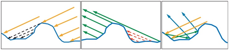
So, we now know what spherical harmonics are, but how are they used to compute the irradiance maps we want? Remember that the texels of the irradiance map are the average of the sky box texel colors over a hemisphere. This produces a very blurry cube map. Well, we can approximate the sky box using low order spherical harmonics, which in turn produces a very blurry cube map that looks strikingly similar to taking the average over the hemisphere.

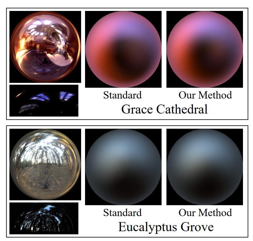This image comes from the paper linked earlier. The “standard” images are made by taking samples over the hemisphere. The “our method” images are created by representing the source cube maps using 2nd order spherical harmonics.

If you were paying attention and also put some things together that I mentioned earlier, you might realize that approximating using low order spherical harmonics is very similar to the low pass filter example I gave earlier. This isn’t a coincidence! We’re basically “low passing” the spherical harmonics of the sky box to produce our diffuse irradiance maps. Here is a picture from my engine:

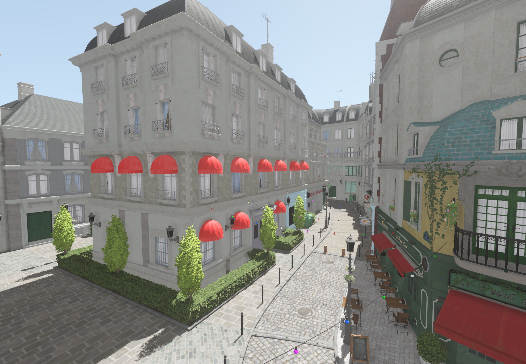Here is a before image with a flat ambient term.

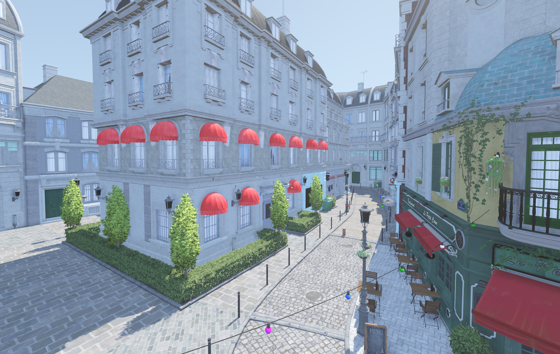Here is the after image with diffuse irradiance. Notice how everything is slightly blue, since it’s reflecting the sky box. Also notice how everything seems to have more depth.

Prefiltered Environment Maps

The comparison picture shows the striking difference between using a constant ambient term and image based lighting. However, something is missing: reflections. That’s because the irradiance maps only compute the diffuse term for the BRDF. It’s especially noticeable with metallic surfaces, since they only reflect light (they don’t have a diffuse term).

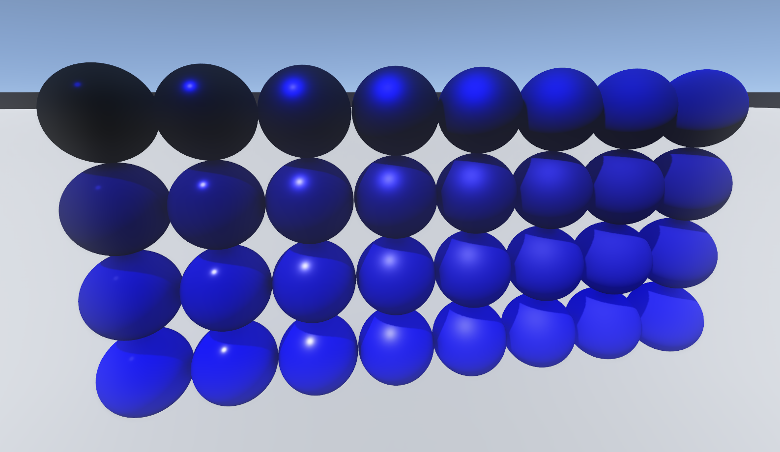From left to right, you go from low roughness to high roughness. Going from bottom to top, you get low metallic to high metallic. Notice how the perfectly smooth, perfectly metallic sphere is completely black since it doesn’t have any light to reflect. Also notice how hard it is to tell the difference between rough and smooth non-metallic spheres.

We still need the specular term. It turns out that computing the specular term is much harder. Why?

1. Smooth surfaces reflect the sky box perfectly, meaning the image isn’t blurry at all. We also need intermediary cube maps for surfaces that are rough but not completely rough.
2. Because the cube maps aren’t completely blurred out, we can’t use low order spherical harmonics. We’d need to use a much higher order, which would defeat the purpose of using them in the first place.
3. Surfaces reflect differently when looking at them at different angles.

The end result of all of this is that we’d need a lot of cube maps and a lot of processing power to compute them in real time. In order to get around this, we use a few techniques. The first is called the “Split-sum approximation” which comes from a presentation on shading in Unreal Engine 4 by Karis. As the name implies, we take the specular portion of the BRDF that we’re trying to solve and split it up into two sums (woah).

The split sum approximation from Real Shading in Unreal Engine 4. The left sum is what we’re trying to solve.

The first sum is called a pre-filtered environment map. It’s a mip chain where each level of the mip chain represents irradiance at higher and higher roughness values. So, the first level is for a completely smooth surface, an the lowest is for a completely rough surface. Unfortunately, we have to make the assumption that we are viewing the surface from directly above (i.e. surface normal = view direction = reflection direction). This means we don’t get cool grazing angle reflections, but it does mean we can do everything in real time, so I call that a worthwhile trade off.

From Learn OpenGL. You can see how the approximation destroys the grazing angle effect.

The second sum is actually a look-up texture. The input is a 2D vector with the roughness in one dimension and dot product between the surface normal and viewing direction in the other. The output is a scale and bias to F0 (Fresnel reflectance at 0 degrees). This LUT can be precomputed at build time.

The second term’s look-up texture.

The end result is nice reflections, like so!

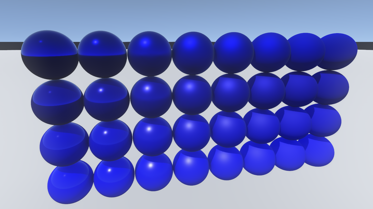Spheres with full image based lighting. Specular reflections make metallic and smooth spheres look much better.

Improving Performance

The naive implementation for specular IBL still requires thousands of samples per texel per mip level, and runs in about half a millisecond for a 256 texel size cube map. That isn’t awful, but we can do better. This article by Padraic Hennessy describes some things you can do to improve performance.

The first thing to do is realize that the first mip level is actually the same thing as the cube map texture you’re sampling, so you don’t even need to take any samples. You can just copy the image directly. Pretty easy!

The second optimization is called “filtered importance sampling.” Importance sampling is related to the integration technique used to create the cube maps (Monte Carlo integration). The idea is that our BRDF has certain directions that are more important than others (specifically, those aligned with the surface normal). Therefore, when taking random samples, we can get away with taking fewer samples by sampling more often in the directions that are “important.” The “filtered” part is about sampling mip map levels instead of the source cube map directly. This allows us to get down to 32 samples per texel, which is pretty amazing!

The last optimization is to precompute the sample directions, weights, and mip levels and look them up while we’re sampling. We can do this by doing the math in a space local to the sample instead of doing everything in world space. All together, the optimizations get us down to a tenth of a millisecond, which is perfect!

Conclusion

All together, image based lighting adds a ton to the realism of a scene. It still isn’t a completely accurate solution for global illumination but it certainly works well enough for these outdoor scenes, as you can see. Although my next area of research is going to be mesh shaders, I’m definitely interested in getting ray traced reflections and global illumination working in my engine.

I hope you learned something, and I hope the resources I linked are useful for doing this stuff yourself. If there are any mistakes you spotted, or you have any questions, please feel free to email me.